Exploding dice is a mechanic that appears in various tabletop games. It works like this: a dice is rolled, if it lands on its maximum values, it “explodes” — the dice is then rolled again, adding the new value to the max value of the dice. If dice again lands on its maximum, the dice explodes a second time. This process continues and may lead to chains of explosions that push the roll total far beyond what is normally expected.

This mechanic appears in a number of tabletop games, with Savage Worlds likely being the most popular system within the RPG space that uses it. In this post, we dig into the infinite nature of exploding dice and explore the math and expected outcomes from this fun mechanic.

Exploding probabilities

Suppose we roll an $n$ sided exploding dice. The probability of rolling a non-exploded value, that is between $1$ and $n-1$ is no different than a normal dice roll. Each face below $n$ appears with equal probability $1/n$. If instead the dice explodes — which happens with the remaining probability $1/n$ — we add $n$ to the outcome of a new exploding dice roll.

Let’s look at an example when we are rolling a 6-sided dice, so $n = 6$. Any result between 1 and 5 appears with probability $1/6$. How about the probability of rolling a 7? Rolling a 7 requires rolling a 6 on the first roll, triggering the explosion, and then rolling a 1 on the second:

Any value of the exploded dice roll can be written like this — as powers of $1/n$. Suppose we want to know the probability of rolling a 25 on an exploding d6. Well that’s just rolling 6 four times in a row followed by a 1, so $p = 1/6^5$. In general, for an $n$ sided dice, the probability of rolling any given value is:

Where $\lfloor{x/n}\rfloor$ represents the rounded down result of dividing $x$ by $n$. The probability of rolling a multiple of $n$ is 0, because every time a multiple of $n$ would show up, it triggers a dice explosion. The below graph shows the outcome probabilities when rolling an exploding d6.

Within a given number of explosions, each outcome is equally likely. As the number of explosions increases, the probability decays rapidly due to the rarity of rolling many 6s in a row. This particular graph cuts off at 18, but in reality it continues to infinity with ever decreasing probabilities.

The probability of at least $k$ explosions on an $n$ sided dice is $P(\textrm{at least k explosions}) = n^{-k}$. Continuing with the d6 example, we have:

While one or two explosions is fairly common, more beyond that are quite rare, with a less than 1-in-1000 chance that you roll at least 4 explosions on a d6.

Explosive expectations

Another way to understand the effect of the exploding dice mechanic is to look at how it changes the average or expected outcome of a roll. In a previous post, we showed that the expectation of a normal $n$ sided dice roll is $(n + 1) / 2$. It is clear that exploding dice would have a higher average, but by how much?

We’ll calculate this by appealing to something called the law of total expectation. It allows us to write the expectation of an exploding dice roll as follows:

By breaking up our expectation into two distinct cases — exploding and not exploding — we simplify our approach. First, the probability statements are are easily addressed by our previous work:

Next, we consider the expected value of a roll with no explosion. Since each outcome below the maximum value is equally likely, this the same as the expected result of an $n-1$ sided roll. Plugging in to $(n + 1) / 2$, we get:

The last term, which is the expected value of an exploded dice is less clear, but we can get around it with a little trick. Recall that once a dice explodes, you can view it as a new exploding dice roll with $n$ added to the final result. We can express this as:

While it may seem odd to write the original thing that we were trying to solve for — $E(X)$ — on the right hand side, it’s perfectly valid to do and will help us later. Now that we have expressions for all four terms in our original expectation equation, we can plug in to get:

The above simplifies to:

We take advantage of our trick by subtracting $E(X)/n$ from both sides to gather all the $E(X)$ terms on the right and solve to get:

Careful inspection of our final result shows that the expectation of a normal dice roll appears on in our result, $(n + 1)/2$. A succinct way to summarize the effects of the exploding dice mechanic is that it increases the expected result by a factor of $n / (n - 1)$.

Revisiting our $n=6$ case, we plug in to see that $E(X) = 4.2$. A notable increase over the normal average of 3.5. The below graph summarizes the differences over the standard dice from d4 up to d20.

While the effect is of a similar magnitude across different types, it is most significant for low-faced dice. The factor of increase, $n / (n - 1)$, quickly approaches 1 as $n$ increases, but with few sides it is relatively large. For a d4, the increase from an average roll of 2.5 to one of 3.33, represents a 33% increase. On the other hand, the d20’s 10.5 to 11.05 increase is a meager 5%. The graph below shows percent increase of the exploding mechanic across the standard dice types:

Despite explosions having a consistent increase the expected outcome, as a percent difference, the effect is attenuated for high-sided dice. Such a difference suggests some reasoning behind the prevalence of exploding dice in d6 systems, but less so in those with a greater d20 focus.

Regardless of those differences, exploding dice is a fun mechanic that leads to some interesting math and meaningfully alters outcomes in systems that employ it.

Rolling for stats in DnD 5e always carries the risk of ending up with a weak character. Despite recommendations to use the standard array, point buy, or any number of homebrew rules for generating stats, rolling rules-as-written nevertheless remains common. For these tables, poor rolls inevitably occur, and when that happens, many DMs implement bad luck protection by allowing bad stats to be rerolled.

In this post, we look at the mathematical consequences of rerolling your stat array. By setting a limit on how bad a player can roll before allowing a reroll — we call that limit the bad luck threshold — the underlying distribution of possible outcomes changes and biases ability scores higher than they would otherwise be.

Reviewing the standard array and rolling RAW

Before we dive into how rerolling changes the odds, let’s review how rolling rules-as-written compares to the standard array. As a reminder, the standard array is [8, 10, 12, 13, 14, 15]. Rolling for stats with 4d6 dropping the lowest generates a wide range of possible outcomes.

The chart below compares the two methods. The top-left shows the distribution of possible outcomes for the lowest value in your rolled array; typical values are somewhere between 6 and 11. The red line at 8 indicates the corresponding standard array values. Moving right, we see the distribution for the next highest stat in the array. This continues until the bottom-right, showing the possible outcomes of the highest stat in the array.

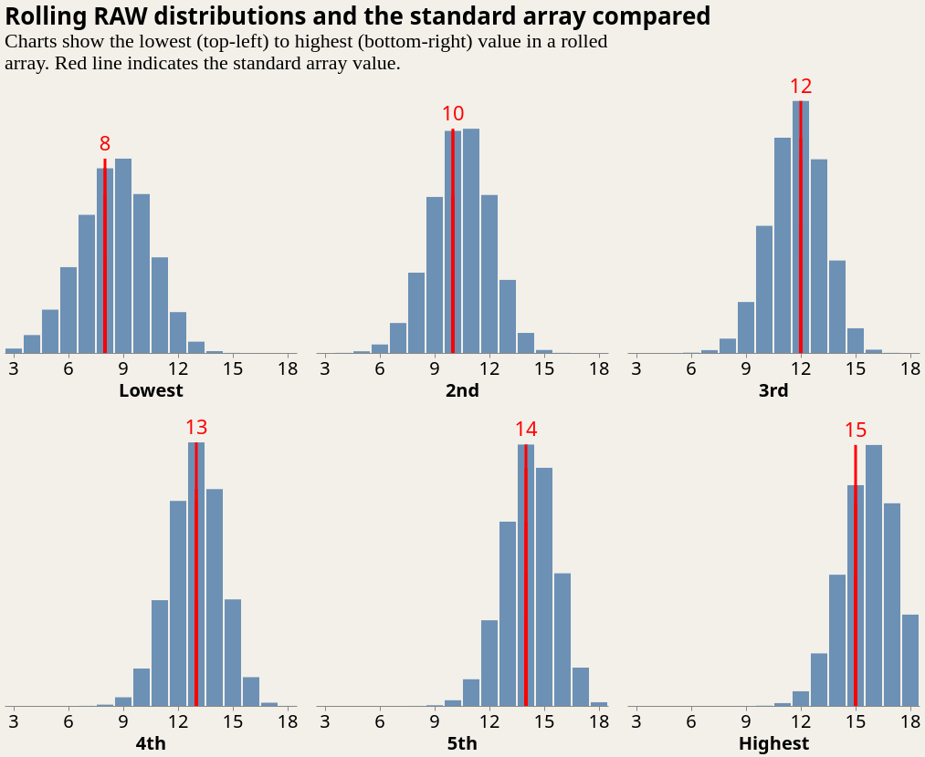
The standard array more or less selects the average from rolling, but not always! Interestingly, the largest deviation is the highest stat — rolling more often than not gives 16 or higher, compared to the standard array’s 15.

Seemingly small differences result in the fact that rolling will on average give higher ability scores than the standard array. By looking at the total ability score of the array, which is sum of the whole array, we get a better idea of how they compare. The figure below shows the bell-shaped curved of the total ability scores from rolling compared to the red line of the standard array.

The standard array’s red line is slightly left-of-center of the potential outcomes from rolling. Compared to the standard array’s 72 total ability score, rolling has an expected value of about 73.5. An extra point or two isn’t earth-shattering, but it is a difference worth noting.

Bad luck protection and the upward bias of rolled stats

Armed with an understanding of how different rules generate differing ability scores for a character (point buy is beyond this post’s scope), we shift our focus to how these rules work in practice.

As mentioned in the intro, many groups rightly prioritize the enjoyment of the players over some arbitrary standard of mathematical fairness by rerolling bad arrays. This biases the total ability score upwards by cutting out extreme lows.

One can imagine that a player who has the misfortune to roll significantly under the standard array may want a reroll. This has the effect of chopping off the left side of the total ability score distribution and increasing the odds of the remaining outcomes.

The chart below shows how that shift happens — the underlying yellow-orange bars represent the full possible outcomes of rolling, whereas the slightly higher overlaid blue bars show how the distribution changes when it gets cuts off. The bad luck threshold shown here is the point where we say “any stats that are worse than this should be rerolled”.

The relatively modest bad luck threshold shown above, where a player rerolls when their total ability score is 60 or below (which are effectively commoner stats!), has the same shape as before, but with the left tail cut off. Although the difference seems minor, it is enough to raise the expected total ability score from 73.5 to 74. By allowing players to reroll commoner-tier stats, they expect to gain half of an ability score in the process.

Every bad luck threshold we pick gives a different expected boost to your ability score.

The figure below shows just how that bonus varies. The horizontal axis represents the different thresholds we can set. Higher bad luck thresholds correspond to being more generous with rerolls. The vertical axis is our expected total ability score when we roll using this bad luck protection rule.

As we increase the threshold, we see our expected stat total increase (as represented by the blue markers). Our previous threshold of 60 puts us right at a full ability score increase above the standard array. Increasing it to a higher value of 68 or so is equivalent to two full ASIs above the standard array.

When phrased in terms of ASIs, it’s clear that rolling RAW already gives a notable average boost over the standard array. Adding even a small amount of bad luck protection to that pushes the disparity even further.

As mentioned previously, a bad luck threshold of 60 — which corresponds to an average ability score of 10 — is enough to push rolling to a full ASI above the standard array. A more generous threshold of 66, or an average ability score of 11, doubles the expected stat bonus of rolling from 1.5 to 3 above the standard array.

Of course, a single number like the total ability score cannot capture all of the nuances that come into play when determining what is a “good” stat array. Having a very strong primary stat can more than make up for a poor dump stat or two, and none of that nuance is appropriately captured by this post. Regardless, when looking at different methods for generating ability scores, it’s important to explore how they are used in practice for an honest comparison between them.

Some thoughts on fairness

There is nothing wrong with ensuring everyone is happy by allowing players to rerolls stats, but tables should be wary as to how this method can affect players that use different stat generating methods. If some players want to roll and others prefer to use the standard array, bad luck protection can lead to a lopsided power balance in favor of the rollers.

On one hand, it is something that could easily go by unnoticed and (in all honesty) likely wouldn’t have too much of an effect on the game. On the other hand, it could feel bad to effectively give an ASI to some players at character creation and not to others. Encouraging everyone to use the same method for generating ability scores ensures an even playing field, but if a table does split, buffing the standard array by an ASI isn’t a half-bad way to go.

Another point that often comes up in these discussions about rolling for stats is the opposite problem — good luck protection. Players who roll far above their party members may feel guilty about their greater character power and choose to reroll to get a more average array. This has a counteracting effect, pushing the expected ability scores lower. One strategy to constrain extreme ability scores is to reroll on both overly weak and overly strong characters. If the reroll rules are symmetric, it leaves the expected stats unchanged from the original method.

The goal of character creation should always be to create a party of adventurers that your table is excited to play. Keeping in mind that something as simple as allowing a player to reroll their stats will inflate them is worth keeping in mind, so that you can ensure balanced table where everyone can shine.

In DnD 5e, a group check is a helpful mechanic to approach situations where the entire party succeeds or fails together. While group checks don’t always come up in the average session, they certainly have their place. In my games, I often use a group Stealth check if the party tries to collectively sneak past an enemy or to adjudicate a Survival check to see if they navigate a hazardous terrain effectively.

Unfortunately — perhaps due to the designers assuming they are rare — the rule determining group checks is very sensitive to whether you have an odd or even number of party members.

Let’s take a look at the rule as written:

To make a group ability check, everyone in the group makes the ability check. If at least half the group succeeds, the whole group succeeds. Otherwise, the group fails. — Player’s Handbook p. 175

The rule itself is simple, but issues arise in the: “at least half the group” clause. As we know, party sizes in DnD are typically somewhere between 3-6 players. If you happen to have an odd number of players in your group, you’re stuck with interpreting what that “at least half” means — do you round up or down?

That decision is best left to the rules lawyers. Instead we focus on the fact that either decision leads to a situation where your party is punished or rewarded just because they have an odd number of members.

The below figure shows what I’m talking about. (Here I assume each party member has a 50% chance of success, which is not necessarily realistic but doesn’t change the result).

Every time you hit an odd numbered group size, the success chance shoots up or down compared to an even sized party, with the direction being determined by how you round. These are the sorts of odd results you end up with when you take a simple rule and combine it with having to round small numbers.

A modification of the rule can alleviate this issue. I propose the following change to the rule as written:

To make a group ability check, everyone in the group makes the ability check. If the group has an even number of members, the whole group succeeds if at least half the group succeeds. Otherwise, the group fails.

If the group has an odd number of members, the DM rolls a dice and records if the result is odd or even. If the DM rolls odd, the whole group succeeds if at least half the group succeeds, rounded down. If the DM rolls even, the whole group succeeds if at least half the group succeeds, rounded up. Otherwise the group fails.

Essentially, we change the rule so that with an odd number of players, the DM randomly chooses between rounding up or down the number of players required for success. This randomization process results in a compromise between the two extremes.

The below figure shows how the proposed rule compares to the original:

The success chance of our new rule is shown in red. It is clearly more well behaved when it comes to odd numbered group sizes. I’d go so far to argue that the proposed rule is more fair to the players — no group should be significantly affected by whether they have an odd or even number of members!

The downside of the proposed rule is that it places a little more burden on the DM by requiring an extra roll, but I believe the added complexity is worth it. Maybe I am the only DM who uses group checks and it doesn’t really matter, but hey, hopefully there was something interesting here to think about.

Calculating damage is a common — perhaps the most common — task in analyzing builds and theorycrafting in Dungeons and Dragons. It is not an easy one, however. Like many other concepts in DnD, damage comes at the whims of dice. For this reason, damage cannot be effective described as a single number, but rather as a distribution of possible values. On top of that, there are a number of rules and spell-specific effects that must be accounted for when determining the range of outcomes.

In this post we’ll lay out the general framework of the damage distribution and calculate it for a basic attack roll.

Describing damage as a probability distribution

When a character attacks or casts a spell there are typically two steps that occur: 1) a roll by either the player or the DM to determine the degree to which the target is affected and 2) a subsequent damage roll that determines how much damage is taken by the target. There is randomness at every step of this process so we can best represent its outcome as a probability distribution $p(d)$, which is the probability that an attack does $d$ damage.

Let’s think about how we can compute this for a standard attack roll. We start by recognizing that a target can be affected by an attack in three ways: a miss, a normal hit, or a critical hit. A miss deals no damage, a normal hit will deal damage as written in the ability block, and a critical hit deals damage but with double the number of dice rolled. These three possibilities can be represented by breaking down our damage into conditional components:

Where $H = \lbrace \textrm{Miss}, \textrm{Normal}, \textrm{Crit} \rbrace$. The above expression states that the probability that $d$ damage is done is the weighted sum of doing that damage under each of our three hit types. By breaking it down like this, we can directly compute $p(d)$ by first looking at the hit probabilities, $p(h)$, and conditional damage distributions, $p(d|h)$.

It’s not too hard to see that this general formula can represent other damage processes. For a spell with a saving throw we could have $H = \lbrace \textrm{Success}, \textrm{Fail} \rbrace$. From there, it comes down to defining the conditional damage distributions.

The hit probabilities of an attack roll

The first step of computing our attack damage distribution is calculating the hit probabilities $p(h)$. We will only concern ourselves with a standard roll, no advantage or disadvantage. Their effects could be explored with the appropriate substitution of probabilities given by advantage or disadvantage rules, and following the structure of the rest of this post.

We’ll start with a critical hit. The rules state a critical hit occurs when rolling a 20 on an attack roll. For a standard attack roll, this is simply:

Next, we examine the probability of a normal hit, i.e. a roll that meets or exceeds a target’s AC after bonuses but is neither a critical hit or a critical fail (which guarantees a miss). To do this, we must reach back to our previous post on dice rolls probabilities.

We introduce two new parameters: a target roll, $t$, and a bonus to add to the roll, $b$. In an attack roll, $t$ is typically the target’s armor class. The parameter $b$ is usually a combination of a proficiency bonus and a stat modifier.

As an example, suppose a fighter with a +5 to hit attempts to strike a Goblin with AC 15, then $t = 15$ and $b = 5$.

If $X$ is the outcome of our attack roll, then we can write:

Using our dice roll probabilities, we can write this as:

The above expression describes the probability that a roll meets or exceeds the target after bonuses, while excluding critical hits and failures.

The last category to look at is the probability of a miss. We could calculate it directly as before, but it’s easier to just derive the result using the complement:

Then we can write:

With this, we fully describe the probability of an attack hitting when accounting for the target’s AC and the attacker’s bonuses. From here, we turn our attention to the conditional damage distributions.

Damage conditional on the attack roll

The damage distributions themselves are determined by the specific attack type or spell being used, but most follow a pattern — the total damage is determined by the sum of rolling one or more dice and adding a bonus. We will write ${}_{m}D_n$ to represent the random variable of a sum of $m$ $n$-sided dice and $d_0$ will be the damage bonus added, then:

With the way we’ve written the above, we can see that our damage distribution can be written directly in terms of ${}_{m}D_n$, which we conveniently defined in a prior post.

For our normal damage distribution, we write it out directly:

Which is the full expression of our dice roll sum distribution equal to $d - d_0$ as above.

Critical hits are a simple modification of the above, substituting $m \to 2m$, which represents doubling the number of damage dice that one rolls. This gives:

Our last distribution — damage when the attack roll is missed — is the simplest:

When an attack is missed, damage done is 0 with probability 1. Simple enough.

Complete damage distributions

We now have all the necessary components to compute $p(d)$ in its entirety. As a reminder, for an attack roll we have:

It would be too verbose to substitute all of our values directly into this expression, but easy enough to describe the output by looking at graphs of different damage distributions. Let’s consider some examples:

Suppose Ria, a fighter, is facing down a zombie. Her attack bonus with her longsword is +5 and the zombie’s AC is 8. Ria’s longsword deals 1d8 + 3 slashing damage. What is the damage distribution of her strike?

From the prompt, we know that $t = 8$, $b=5$, $m=1$, $n=8$, and $d_0 = 3$. All there is to do now is plug these values into our previously described expressions. The below graph shows the probable outcomes of her strike.

It’s not exactly a bell curve to say the least. The complex behavior is the mixture of our three possible damage conditions — the single bar at 0 is the probability of missing, the mostly uniform damage from 4 to 11 is the damage from a normal hit, and the triangular distribution that lies on top of that is the critical hit damage.

The shapes and relative magnitudes depend on all the parameters present. To see just how different they can be, let’s consider another situation.

An adventuring party is going toe to toe with a large Ogre. Yar, a cleric, calls on the power of his deity to cast Inflict Wounds at 1st level. His spellcasting ability modifier is +5 and the AC of the Ogre is 11. Damage dealt on a hit is 3d10 necrotic damage. What is the damage distribution?

We approach this in a similar way to before, noting that $t = 11$, $b=5$, $m=3$, $n=10$, and $d_0 = 0$.

Now we see an entirely different distribution. The 0 damage possibility has risen to 25% and the bulk of the non-zero damage forms a familiar bell curve from the 3-dice sum with a long tail that represents possible crit damage.

In both of these examples, the mixture of different attack roll outcomes gives rise to non-trivial damage outcomes. Even so, the damage from an attack roll that we explored here is one of the simplest damage mechanics in 5e. Varying spell effects, different damage types, and other features all paint a rich mechanical picture. It suffices to say that we still have much to explore in this realm, but that will be for future posts.